 |
Beating The Atmosphere
Have you ever wished you were in Hawaii? Tropical seas, warm weather, Luau's and (most critically), some of the worlds biggest telescopes on a very high mountain tops -- because of the good atmospheric seeing. In comparison, we're stuck with Durham. Rain, cloud, and even when it's clear, strong turbulence. Perhaps all is not lost. Perhaps we can take observations that are as good as those from Hawaii, but only for a very short time.

The goal of this project is to measure the properties of the atmosphere above Durham on a "typical" night (or nights). Is it possible to image stars at a rate where the atmosphere is "frozen", and so get close to the diffraction limit of a telescope? And if so, what is the trade off between image quality, depth, and how are observations of interesting astrophysical phenomenum (e.g. close binaries) affected, and can you test this? There are two approaches for this project. You can undertake one, or both.
1. Lucky Imaging
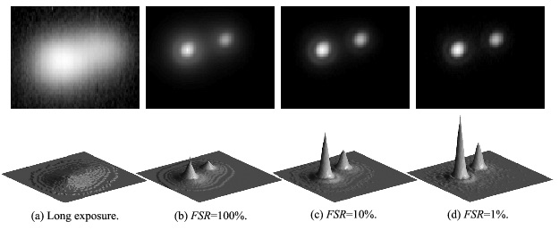
Lucky Imaging is a remarkably effective technique for delivering near-diffraction-limited imaging on ground-based telescopes (e.g. Law et al. 2006 ). The basic principle is that the atmospheric turbulence that normally limits the resolution of ground-based observations is a statistical process. If images are taken fast enough to freeze the motion caused by the turbulence we find that a significant number of frames are very sharp where the statistical fluctuations are minimal. By combining these sharp images we can produce a much better image than is normally possible from the ground.
The term "Lucky Imaging" came from Fried (1978) though the first calculations of the Lucky Imaging probabilities were first carried out by Hufnagel in 1966 and these principles have been used by astronomers to take very high quality images of bright objects. Background on the Lucky Imaging technique can be found here.
The goal of the project is to use the Lucky Imaging camera to determine the fraction of time that the seeing is better than X arcseconds (X=1arcsecond is the typical limit employed by observers in Hawaii). Here are some suggestions for objective you may wish to consider.Familiarise yourself with the camera and its operation. You will need to be able to adjust the exposure time, gain and field of view.
In the lab, take a few images at different rates, and become familiar with how and where the data is stored (be careful: it is possible to generate 1Tb of data in a few seconds!).
The images are likely to be read noise limited, so devise a method to measure the readnoise.
On the telescope, take a series of images of a star (or stars). You will probably want to take several 1000 images with different exposure times, ranging from 1 to several 10's of milliseconds.
Analyse each set of observations. We will need fit the star in every image with a two-dimensional Gaussian profile and record the x/y center, sigmax, sigmay, intensity of the fit (the astrolab "lucky.py" code will automate this, but measure a few images by hand to check its doing something sensible). The seeing is usually measured in terms of full width at half maximum (FWHM). FWHM=2.35 x sigma.
Plot the distribution of FWHM for each exposure time, and also the cumulative FWHM as a function of exposure time. Is there an optimal exposure time?
What fraction of the observing time is the seeing better than 1"?
Shift and add all the images as a function of seeing to create a stack. (e.g. stack the top 1%, 5%, 10% and 50% of the images). How do the images compare in terms of seeing FWHM? A good target for interesting results is M42.
2.Turbulence Profile - The Differential Image Motion Monitor (DIMM)
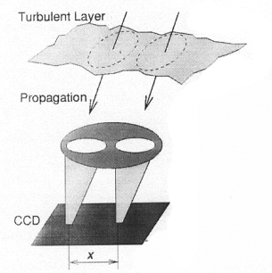
Turbulence in the atmosphere randomly distorts the plane wavefronts from stars. Over a short distance, the corrugated wavefront can be considered approximately planar. The Fried parameter, r0 indicates the length over which the wavefront can be considered planar. As we can see from the figure below, the Fried parameter is also approximately equal to the size of the turbulent cells themselves.The larger the Fried parameter, the better the atmospheric conditions. At a good observing site, the Fried parameter has a typical value of r0=10cm, at an optical wavelength of 500nm. The coherence time is the average time over which the distorting wavefront is coherent. The turbulent cells responsible for distorting the wavefront generally evolve on long timescales. The reason the wavefront changes between time t1 and time t2 is because the wind moves the turbulent cells across the sky.
A measure of the timescale on which the wavefronts change is the time taken for a turbulent cell to move it's own size; the coherence time. The coherence time is given by t0=t2-t2=r0v, where v is the wind speed. At a good observing site on a typical night, v=10m/s and r0=10cm at optical wavelengths. Hence t0~10ms.
To measure the seeing, we can use a differential image motion monitor (DIMM). The DIMM is used extensively at major observing sites (e.g. at the VLT on Paranal, and a description can be found here). In a DIMM this system, two images of the same star are created on a CCD, corresponding to light having travelled through two paralled columns in the atmosphere (see Vernin et al. 1995).
Familiarise yourself with the camera and its operation. You will need to be able to adjust the exposure time, gain and field of view, and store the images as fits files.
In the lab, take a set of images, and become familiar with how and where the data is stored.
The images are likely to be read noise limited, so devise a method to measure the readnoise as a function of gain and exposure time.
On the telescope, take a series of images of a bright star with the mask on. The mask comprises a hartmann hat with two holes, one of which has a wavepl ate which is used to create a second image of the star, slightly shifted. Each image should look like this:
 You will probably want to take several 1000 images with different
exposure times, ranging from 1 to several 10's of
milliseconds.
You will probably want to take several 1000 images with different
exposure times, ranging from 1 to several 10's of
milliseconds.Analyse each image in each set of observations. A Python code to help you is available here. This code (which you will need to edit) fits each of the stars in every image with two-dimensional Gaussian profiles, and for each star records the x/y centers, sigmax, sigmay, intensity of the fits.
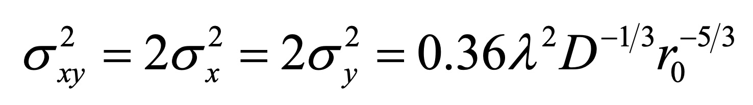
Plot the radial offset from the center of the image as a function of time for each of the two stars. We need to remove the drift (this is caused by the telescope tracking), and then measure r0 using the equation above.
How does the coherence length compare to other observing sites around the world? What is the minimum diameter of telescope that is useful in Durham?
-
How does the seeing you infer from the DIMM compare to the seeing measured from the telescopes using the CCDs for observations taken at the same time?
| Back to the AstroLab Home Page | ams | 2019-Feb-09 13:28:13 UTC |