Durham Postgraduate Data Reduction Course
TimetableLectures are held in OCW017. Practicals will be in the computer rooms CM001 (maths building) and ER156 (Elvet Riverside) -- check the timetable.
Any issues, see Mark Swinbank (OCW113) or Julie Wardlow (office OCW111).
Longslit Spectroscopy
Lecture Notes
The notes from the lecture are available here.
Basic Intro
When we receive spectroscopic data from the telescope there are many steps of data reduction to be done. These include some of the steps that are also done for imaging, i.e., bias-subtraction and/or dark frame subtraction and flat fielding. However, we also need to make sure we have a good wavelength solution (i.e., we know which x-axis pixel corresponds to which wavelength). This requires an image of an arc-lamp (such as Argon) which has strong emission lines of known wavelengths. We can then create a wavelength solution using this information. We will also need to correct for the filter response (i.e., the light through-put as a function of wavelength) and flux calibrate our spectra (i.e., convert counts to flux density) by using observations of a standard star that has a well known flux density at each wavelength.
To get you used to the general steps of reducing spectra, during the workshop you will reduce some longslit data. Most telescopes now have automated pipelines to do most (if not all) of the steps of data reduction for you. However, these "black boxes" are fine until they go wrong. It will be a useful exercise to understand each individual step, so you can then be aware if your data is not reduced properly and where the mistakes may have occured. Therefore, as for the imaging we will be using our friend IRAF. You should reduce the data during the workshop and then do the problem questions to be handed in (deadline: Friday 24th November 2017). The data you're being given is longslit data of an extragalactic nebula which hosts an ultra luminous X-ray (ULX) source. You will therefore obtain a spectrum of both the host nebula and the optical counterpart of the ULX.
The Data
You should have already downloaded and unpacked the data (www.astro.dur.ac.uk/~knpv27/outgoing/pg_dr_spec.tar.gz). This is Gemini-GMOS longslit data of a ULX inside a nebula. This consists of science data (i.e., the object of interest) with corresponding calibratations and standard star data with corresponding calibrations. Science: The science frames were taken in a 3-position dither pattern (two frames taken at each position) to take into account there are gaps between the three CCD chips on the detector. Therefore there are six science frames which come in three pairs (named: 1a,1b,2a,2b,3a,3b). Each pair has a corresponding flat field and arc lamp. The arcs and flats are already reduced for you and are ready to use. The one bias frame can be used for all of the science frames. Standard: There is one observation of the standard star and one corresponding flat field and arc frame. The flat field and arc frames are ready to use and the standard star frame has already been bias subtracted.
The HST colour image of the nebula showing the position of the slit (red
rectangle) and the position of the ULX (circle):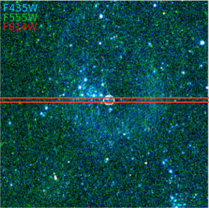
An narrow-band [O III] image of the nebula showing the position of the slit (red
rectangle) and the position of the ULX (circle):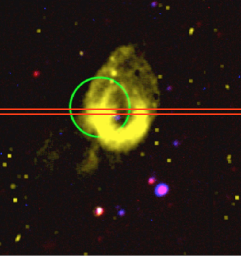
Reduction Steps
You will reduce the data for for the science object first. These are in the "science" folder.
1. Subtract the bias frames off all of the six science frames using imarith
2. Divide all of the bias-subtracted science frames by the corresponding flat field using imarith
You now need to create a wavelength solution for the science frames. You will need to create three wavelengths solutions (one for each arc frame). In IRAF navigate to the package: twodspec.longslit
3. Run identify on each of the three arc frames (i.e, arc1.fits, arc2.fits, arc3.fits). This will use a database of emission lines for the CuAr lamp that was observed (you have been given: CuAr_GMOS.dat) to identify the emission lines in the arc image. Unfortunately you need to do some of this by hand. Make sure that you change the appropriate parameters of identify using "epar identify". Because you will be running this on three separate arc frames, make sure that you give the databases unique names. When you are running identify you will use the cursor to hover over line, press 'm' and then type in the wavelength of that lines. You will need to look at the file "CuArB600_430.eps" or "CuArB600_430.pdf" to find the wavelengths of some of the brightest emission lines (n.b., the raw frames may have an x-axis with *decreasing* wavelength). You should do this for around 10 lines across a wide wavelength range. Then press 'f' which attempts to fit a wavelength solution. You will see the residuals. These should all be within ~<0.5 angstroms. You can delete points you do not like using 'd' and then refit using 'f'. As a final check press 'q' to get back to the screen for identifying lines and press 'l' to see where iraf thinks all of the lines should go. When you are happy press 'q' again and make sure that you say 'yes' to save the output.
Identifying ~10-15 lines by hand: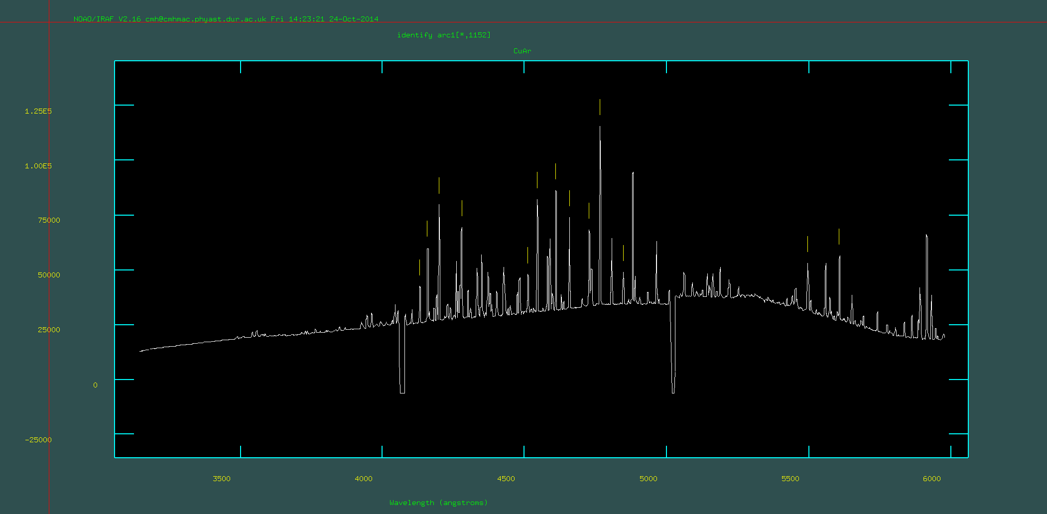
Pressing 'f' to perform the fit and check residuals. Dodgy points
can be removed here: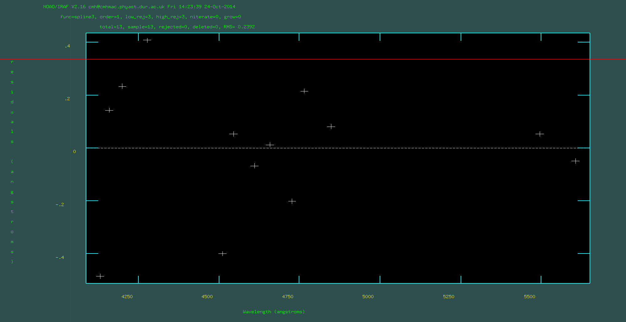
Pressing 'l' on the main screen to check all of the lines. If
this looks bad, start over: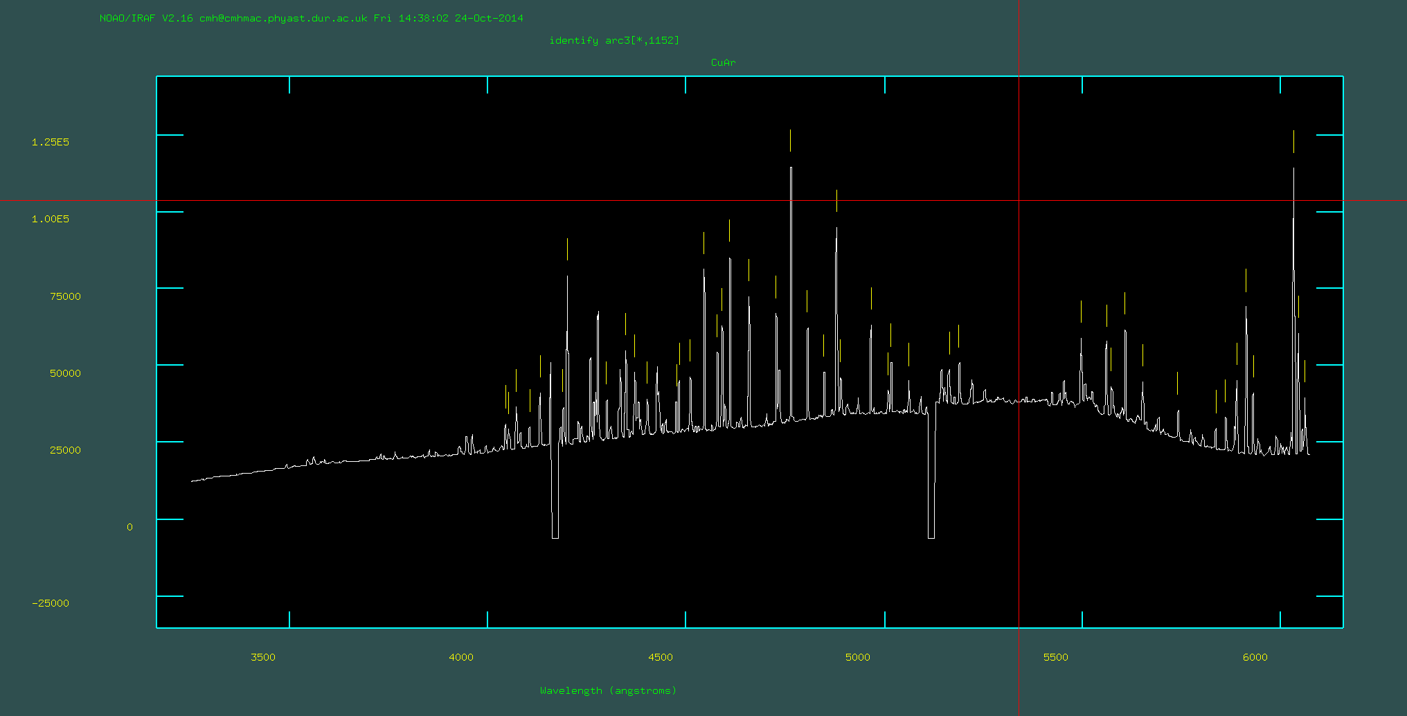
4. Run reidentify on each of the three arc frames. Now that you have identfied the arc lines you need to trace these over the 2-dimensional frame (n.b., you will notice there is some curvature in these lines if you open up the raw arc frames!). You do this with reidentify. Use "epar reidentify" to update the input parameters (use "help reidentify" if you do not know what these are; tip start with nlost=30, nsum=30, cradius=10 and don't forget to change the co-ordinate list and inputs). For this exercise, you probably don't want to run this interactively but you can check it all worked by visually inspecting the frames after step 6. Be careful to use the correct filenames for the input/outputs for each of the individual arc frames. If you need to re-run this routine make sure that you set "overrid=yes" or delete the outputs first.
5. Run fitcoords on each of the three arc frames. Now that you have traced the 2-dimensional arc lines, you need to create the fit that can then be applied to multiple frames (including the science frames). You do this with fitcoords. Use "epar fitcoords" to set the inoput parameters. Again, being careful to use the correct inputs for each of the individual arc frames. Note: you should not include the ".fits" at the end of the input name and input image.
6. Run transform on each of the arc frames. You can now apply the fit that you have created to different frames to give them a wavelength solution (i.e., assign a wavelength to every pixel) and correct for the curvature. You do this with transform. You will first do this on the arc frames to check that everything has worked properly. At this point it will be useful to put all of the frames onto the same wavelength solution, therefore when using epar, set x1=3500, x2=6100, dx=0.5 (check what these parameters do!). Once you have applied transform to the three arc frames, open them in ds9 or GAIA to check that: (1) the emission lines are now straight; (2) there is a sensible wavelength assigned to each pixel (check by hovering over with the mouse). If something looks odd you may have incorrectly identified lines in identify or you may need to change the parameters of reidentify (e.g., experiement with trace=yes and trace=no).
Example arc frame before transform is applied:![]()
Example arc frame after transform is applied. Notice that the arc
lines are now straight but the chip gaps are curved:![]()
7. Run transform on each of the bias-subtracted and flat-fielded science frames. Make sure that you use the corresponding arc frame fit in each case. Also make sure that you give the same wavelength solution to each frame by setting x1,x2,dx. This will mean that you can easily stack the frames later. Check that the sky lines are now straight in each of the science frames and that the wavelength solutions have been applied.
Example science frame after transform is applied:![]()
You now need to remove the sky emission (sky continuum and OH emission lines) from the science frames.
8. Run background on all of the science frames. You can run this in non-interactive mode by using the "sample" parameter. You should sample the sky above and below the spectrum in the science frames. Chose a range that definitely doesn't include any science flux but is reasonably close to the spectrum. You may want to use the "low_rej" and "high_rej" parameters do reduce the effect of pixels that have been hit by cosmic rays. Make sure you change the axis parameter! This can run very slowly. You have two options: (i) keep this running in the background and skip to step 10 while you wait; (ii) write your own python/IDL script that does the same job but quicker.
Example science frame after I applied background. Notice that the
sky lines have now gone (except from some residuals around the
birghtest lines):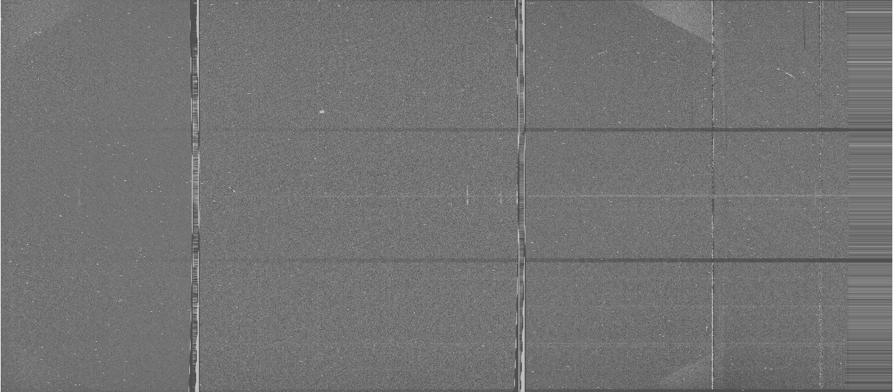
You now need to take the 6 science frames that you have reduced and stack them. This increases signal-to-noise and reduces the problem of cosmic ray events.
9. Stack the science frames using imcombine. Remember that a dither pattern was applied when the observations were taken and therefore we can not stack them "blindly". The astrometry and wavelength solution of the science frames is stored in the header of the fits files. imcombine allows you to apply an offset pattern using this header information. Make sure that you use the appropriate parameter to do this (as always, if in doubt type "help imcombine", tip: look up the "offsets" parameter). You can stack using different methods with imcombine (e.g., median, mean) and with different algorithms to reject bad pixels. A good first guess is to stack using combine=median, reject=sigclip, lsigma=3, hsigma=3. This is median stack with a 3-sigma clipping threshold. In real situations you may want to experiment with different stacking methods.
Example stacked science data: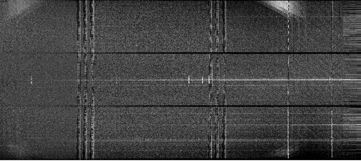
Optional: You should have a frame that looks "clean" of cosmic ray events and the signal-to-noise of the emission lines should be much higher than in the individual science frames. However, you will notice that we can still see the effects of the chip gaps in the stacked frame (the six broad vertical stripes) and sky line residuals (the two narrow vertical stripes). The latter of these can be quite challenging to remove completely; however, it is trivial to remove the effects of the chip gaps. We do this by "masking" the chip gaps in each frame before we stack them. Before we stack the frames we can set the pixels inside the chip gaps to an extreme value like -9999. You could do this in idl/python, or using the command line "setpix" which is part of the wcstools package (google it). Once we have done this on all of the frames, we can re-run imcombine but set the parameter "lthreshold" or "hthreshold" to ignore the extreme values.
A cut-out of example stacked science data when I masked the chip gaps
(much prettier, but also this would be important for real science as
one of the chip gaps was very close to one of the emission lines):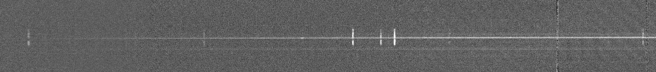
We now have a reduced two-dimensional science frame. However, the frame is still in units of "telescope counts". We want to convert this into flux density units. To do this we need observations of and calibrations for a standard star. You already have these in a folder called "standard". The star that was observed is called: bd284211 or BD+28 4211 (you will need to know this later).
10. Do steps 2-7 for the standard star observation (it is already bias subtracted and the background is negligable for our purposes) so that we have a standard star observation that is reduced, with a wavelength solution.
Example reduced standard star frame: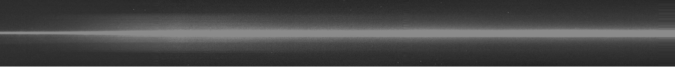
We now need a one-dimensional spectrum extracted from the two-dimensional frame of the standard star. We will use this to find a solution for converting counts to flux density as a function of wavelength.
11. Run apall on the reduced standard star frame. This can be found in the package twodspec.apextract. Choose a suitable output name and set apertur=1. You will run this task interactively. This routine will identify an apperture using the central few columns and then trace the spectrum across all of the columns (i.e., in the wavelength direction). You need to ensure that a suitable apperture has been chosen to get all of the flux of the standard star. In interactive mode: to delete an apperture use 'd'; to ceate a new one use 'm', to change the upper and lower bounds of the apperture use 'l' and 'u'; to remove the sky appertures hit 'b' and the delete them with 't' (we don't need to worry about this small effect here); when you are happy with the apperture press 'q'. Select (yes) to the options that it gives you when you press 'q' so that we can fit the trace interactively. Change the order of the fit to the trace by typing e.g. ":order 4" and hit return. Then type 'f' to refit. Press 'q' when you have finished and view the extracted spectrum.
Defining the extraction apperture in apall: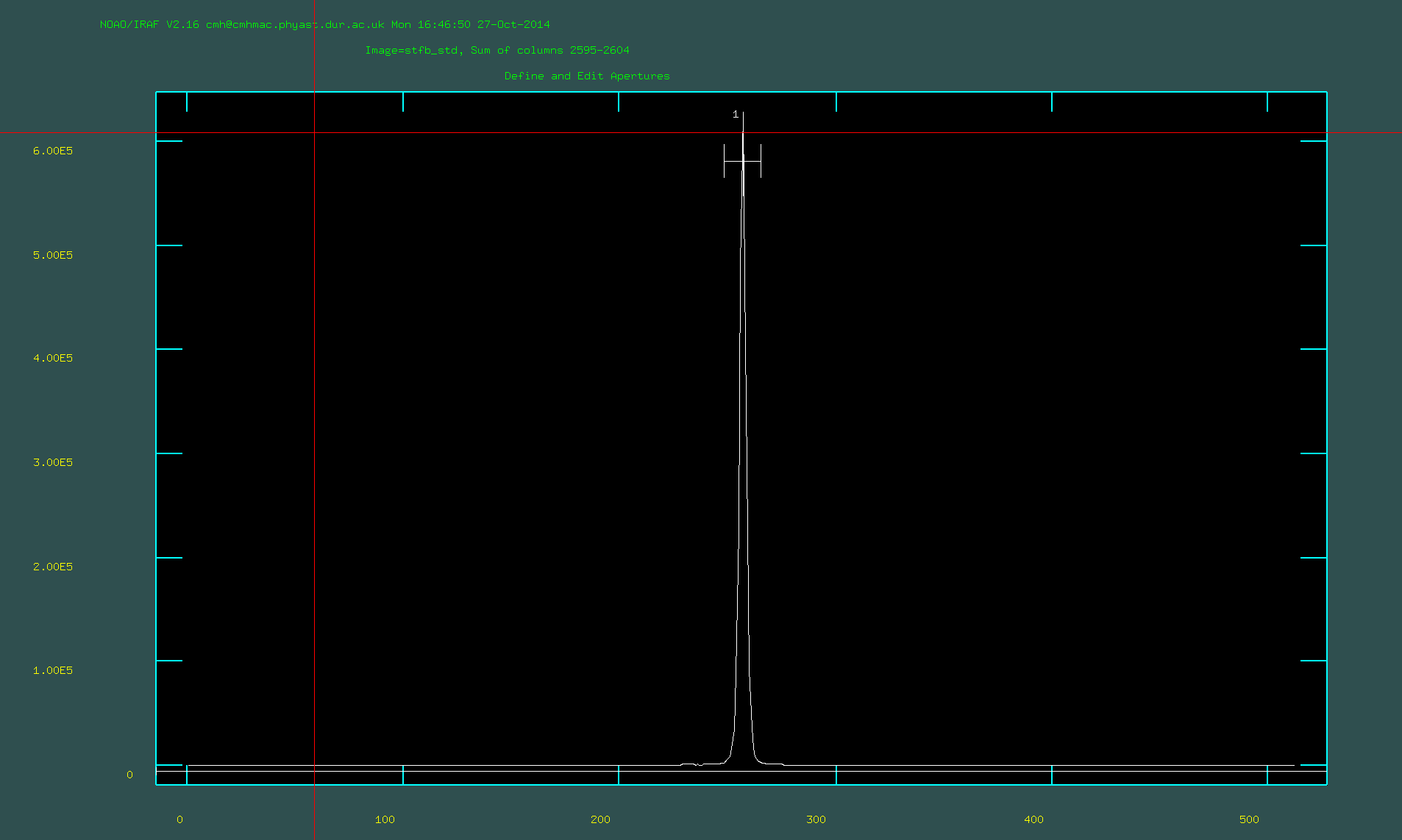
Fitting the trace function in apall with order 4: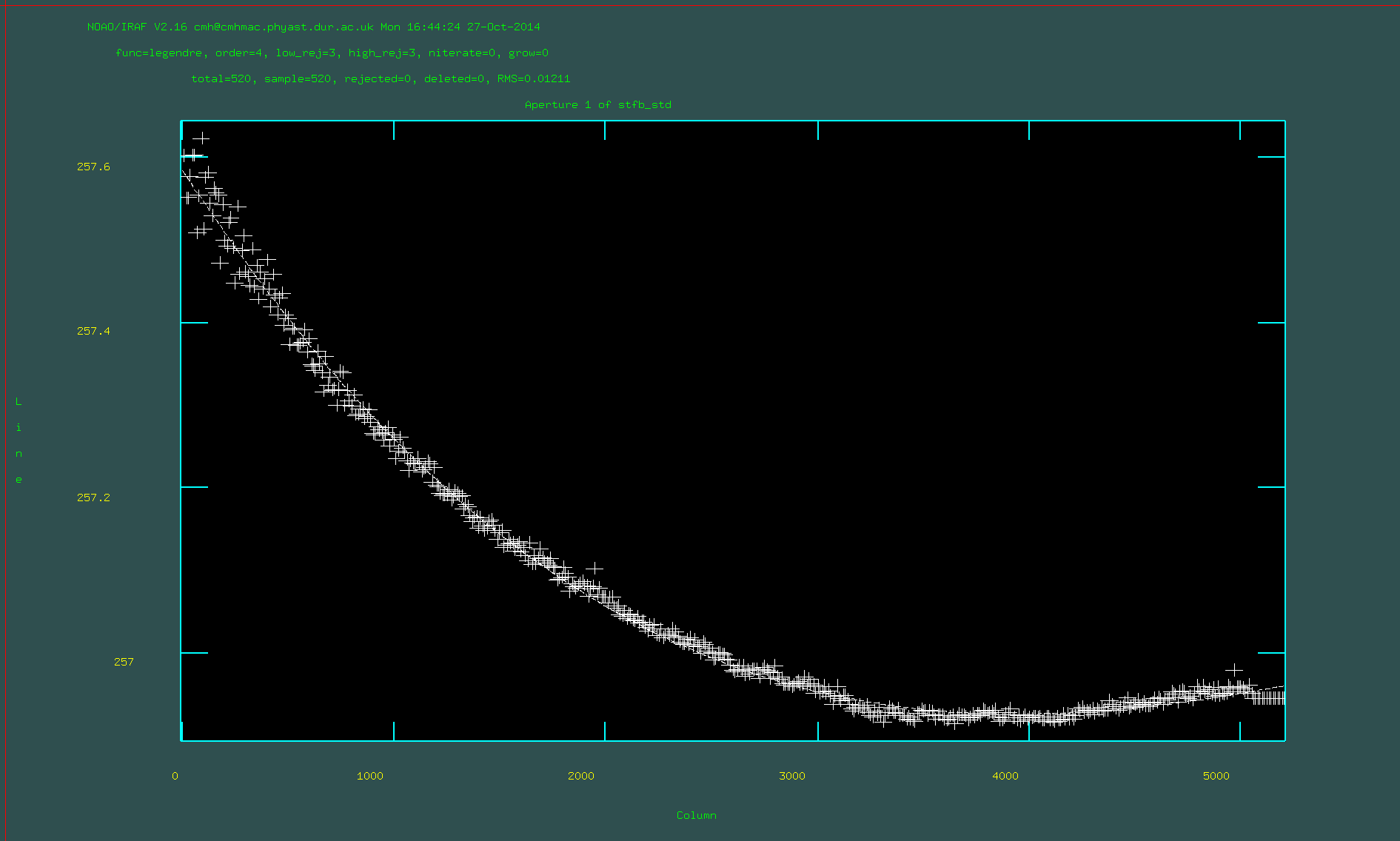
The extracted one-dimensional spectrum of the standard star: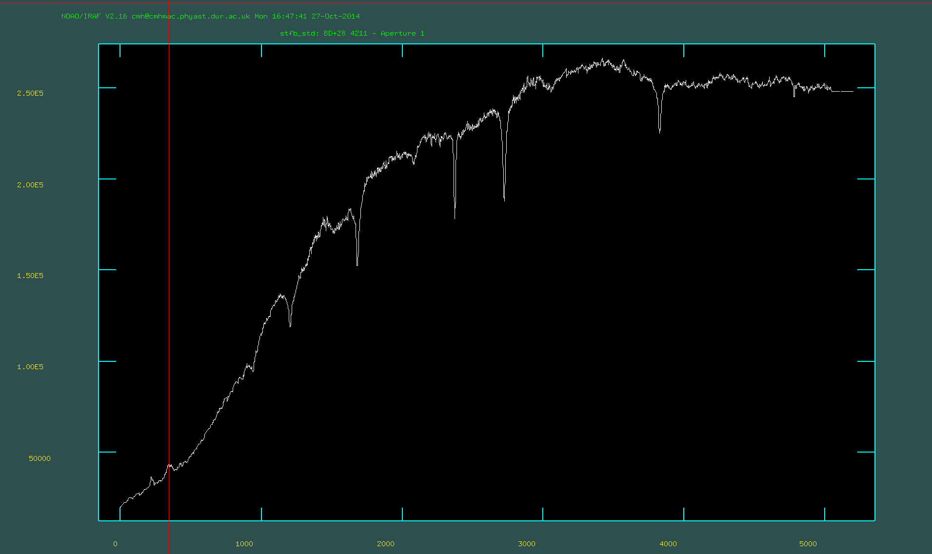
We now have a standard star spectrum in counts. It is useful to have this in "counts per second". However, be careful if doing this on other data! If the exposure time is in the header, some IRAF routines will read the header and ignore the fact you devided by the exposure time.
12. Devide the standard star spectrum by the exposure time (in this case it is 90s) using imarith.
We now can used the standard star spectrum to convert counts to flux density as a function of wavelength. Firstly we need to create a data file for the observations of the standard star using standard (this is in the package called onedspec). Secondly we want to determine the sensitivity function using sensfunc. Finally we can apply the sensitivity function to our spectra using calibrate.
13. Run standard on the one-d spectrum that you have already normalised to 1s. The observatory was Gemini-North, leave airmass=1. The exposure time is now 1s (because we devided by the exposture time); however, note that this parameter is *ignored* if the exposure time is in the header. You will need to point to the directory that contains the model spectrum of the standard star. You can find which directory this is by typing: page onedstds$README (there multiple options to choose from). You don't need an extinction file. You should select "yes" to edit the bandpass interactively. You should check that everything looks sensible and press 'q' when you are happy.
Running standard in interactive mode: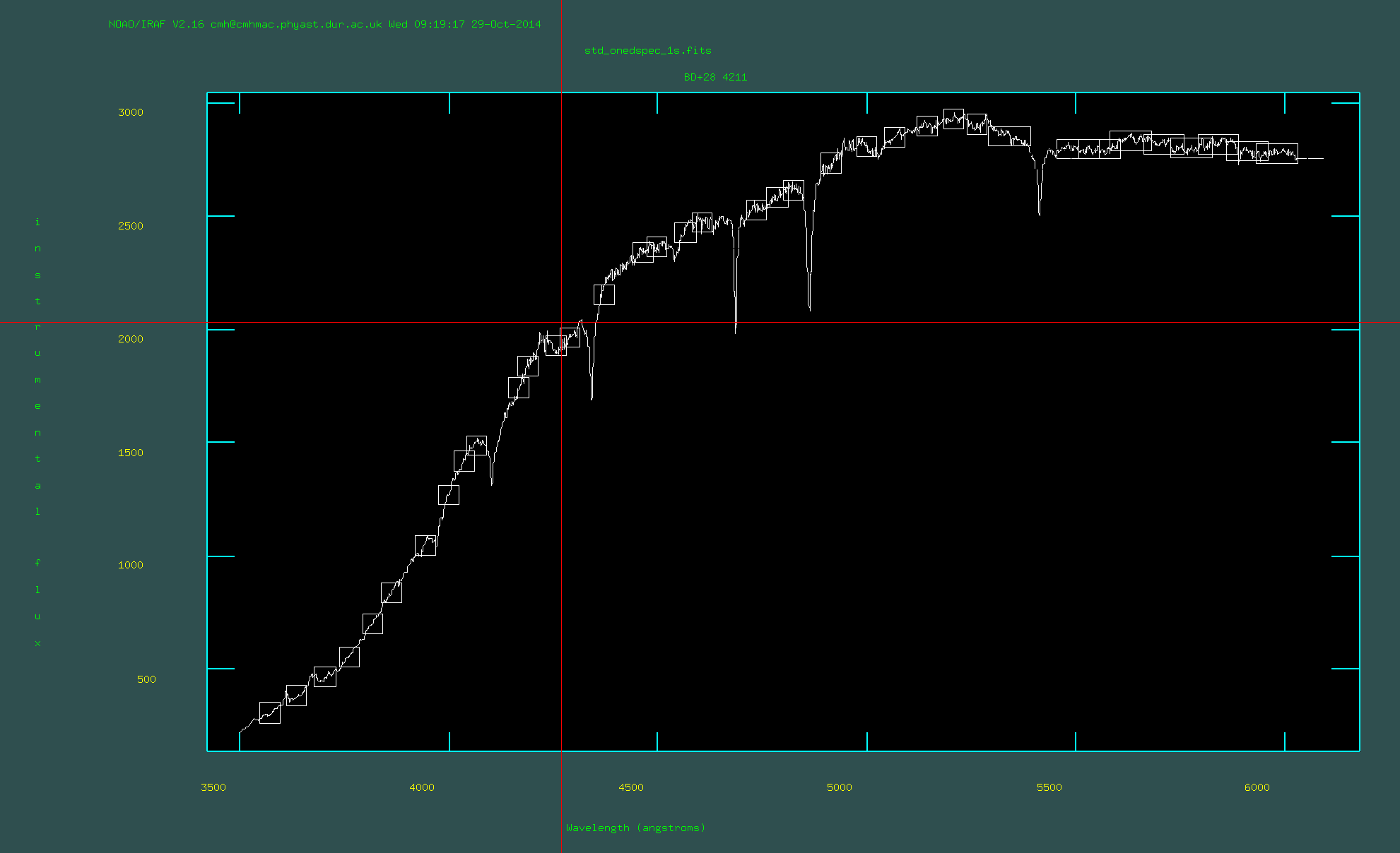
14. Run sensfunc on the file that you created using standard. You should run this interactively to check that the model of the sensitivity curve looks sensible. Sometimes it can be useful to remove bad points by pressing 'd' or adding new points pressing 'a' before re-fitting by pressing 'f'. You can refresh the screen by pressing 'r'. In particular the edges of the wavelength range can often cause a problem.
Running sensfunc in interactive mode: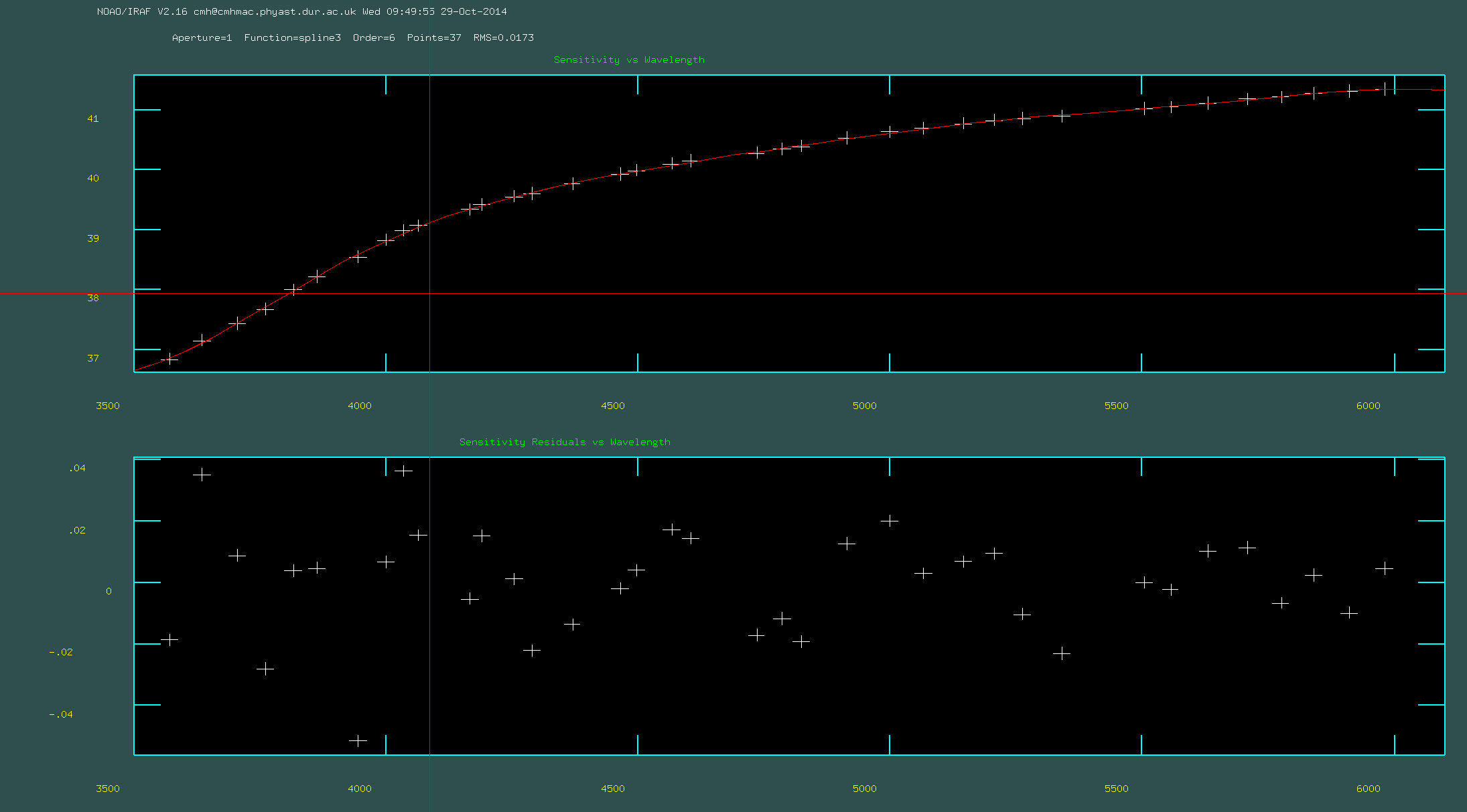
15. Run calibrate on the standard star. This will turn counts into flux density units. Check that the output looks sensible by using splot to plot the spectra (this is also in the package called onedspec). At this point it can be sensible to find a published spectrum of the star, or to check that the flux density values are broadly correctly based on the magnitude of the star and using the NICMOS units converter (http://www.stsci.edu/hst/nicmos/tools/conversion_form.html).
Flux calibrated standard star: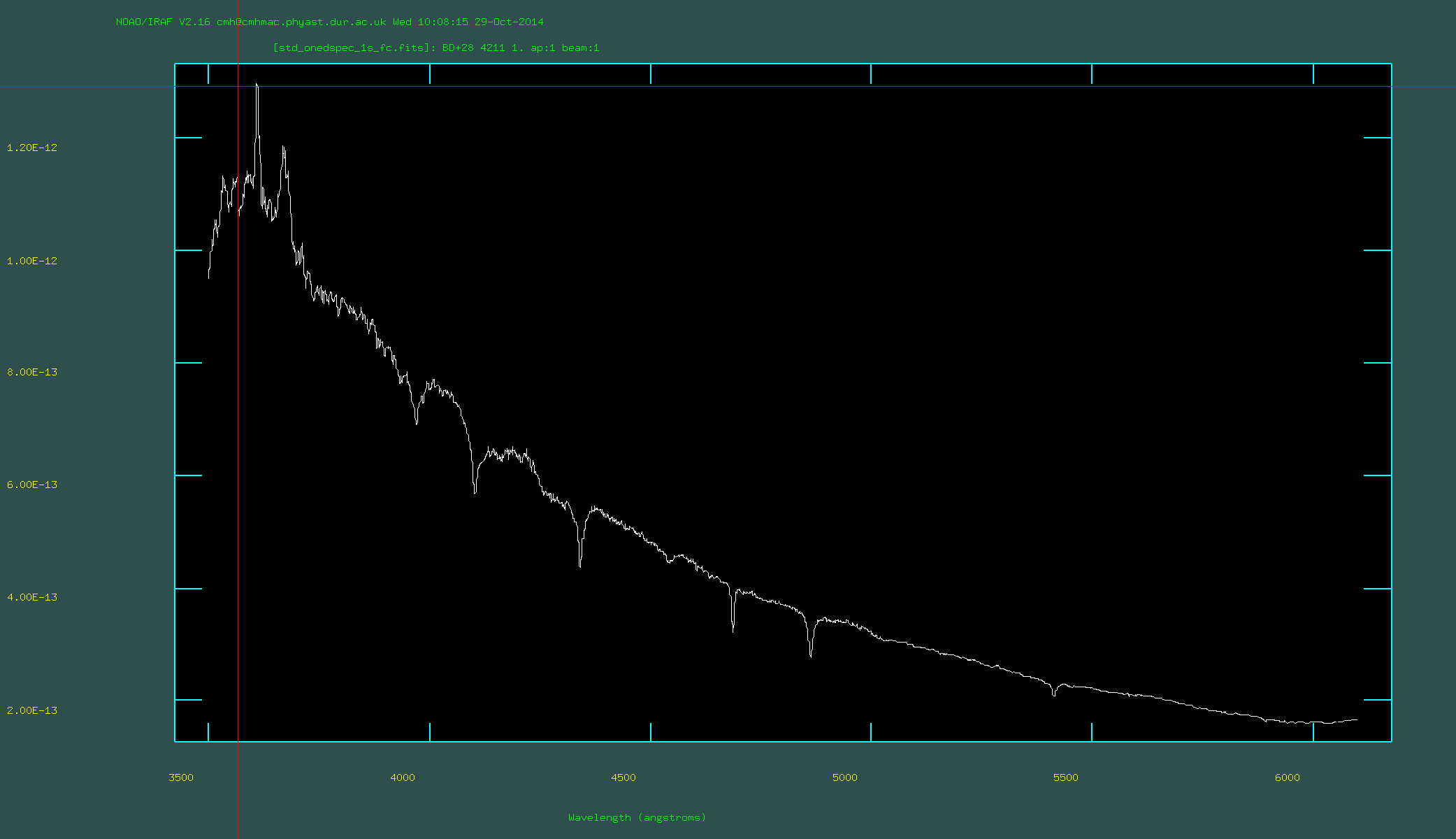
You now have everything that you need to make fully reduced and flux calibrated science spectra (note that the exposure time of the science frames are 919s). You will recieve marks for completing the reduction. You should now do the hand-in questions which should be put into a document (preferably a PDF document) and sent to Julie (julie.wardlow@durham...) & Mark (a.m.swinbank@durham...): before Friday 24th November 2017. You will be asked to present these answers in the lecture on this date.
Hand-in Questions:
For some of these questions you will need to make use of other IRAF rountines (such as splot) that we did not cover in the workshop, or use your favourite programming language. You may need to do some research to find out how to do some of these tasks.
- Show a screen shot of the reduced two dimensional science frame. Label key features, including the data, noise and artifacts.
- Using IRAF/apall (or your own routines in e.g., Python/IDL) extract and plot the spectra of: (1) the region around the star (i.e., dominated by the ULX counterpart) and (2) the whole nebula, in flux density units between 4000A and 5200A. Identify the brightest emission lines of Hgamma, Hbeta, HeII and [OIII] on the plots.
- Measure the noise (i.e., rms) in both of the spectra.
- What is the central wavelength, integrated flux and line-width (FWHM in angstroms and km/s) of the [OIII]5007 and Hbeta emission lines? Comment on whether these measured line-widths represent the true instrinsic line-widths?
- Measure these three quantities for the HeII4686 emission line (produced by the ULX counterpart).
- What are the velocity offsets of the [O III]5007, HBeta and HeII emission lines with respect to rest (HINT: the wavelengths are calibrated to the rest wavelengths in air as opposed to vacuum)? Therefore, what is the velocity offset between the star/ULX and the nebula? Can you give a sensible uncertainty on this value? Show your calculations.